"$1Daddefmas" 修訂間的差異
| (未顯示同一使用者於中間所作的 3 次修訂) | |||
| 行 3: | 行 3: | ||
$1Daddefmas |
$1Daddefmas |
||
I_effective_type |
I_effective_type |
||
| − | <math> m_{hh,z} ~~ m_{hh,x}~~ m_{hh,y}~~m_{lh,z} ~~ m_{lh,x}~~ m_{lh,y} ~~m_{e,z} ~~ m_{e,x}~~ m_{hh,y}~~N_{valley}..</math> |
+ | <math> m_{hh,z} ~~ m_{hh,x}~~ m_{hh,y}~~N_{valley}~~\Delta E_{hh}~~m_{lh,z} ~~ m_{lh,x}~~ m_{lh,y}~~N_{valley}~~\Delta E_{lh}~~m_{e,z} ~~ m_{e,x}~~ m_{hh,y}~~N_{valley}~~\Delta E_{c1}..</math> |
| − | <math> m_{hh,z} ~~ m_{hh,x}~~ m_{hh,y}~~m_{lh,z} ~~ m_{lh,x}~~ m_{lh,y} ~~m_{e,z} ~~ m_{e,x}~~ m_{hh,y}~~N_{valley}..</math> |
+ | <math> m_{hh,z} ~~ m_{hh,x}~~ m_{hh,y}~~N_{valley}~~\Delta E_{hh}~~m_{lh,z} ~~ m_{lh,x}~~ m_{lh,y}~~N_{valley}~~\Delta E_{lh}~~m_{e,z} ~~ m_{e,x}~~ m_{hh,y}~~N_{valley}..~~\Delta E_{c1}</math> |
... to N layers |
... to N layers |
||
| − | I_effective_type is the input type. The default should be 1. The typical semiconductor material has heavy hole, light hole, and electron effective mass of direct band. The type 1 is used. |
+ | I_effective_type is the input type. The default should be 1. The typical semiconductor material has a heavy hole, a light hole, and electron effective mass of a direct band. The type 1 is used. |
| − | For I_effective_type= 1, |
+ | For I_effective_type= 1, m_{hh,z} ~~ m_{hh,x}~~ m_{hh,y}~~N_{valley}~~\Delta E_{hh}~~m_{lh,z} ~~ m_{lh,x}~~ m_{lh,y}~~N_{valley}~~\Delta E_{lh}~~m_{e,z} ~~ m_{e,x}~~ m_{hh,y}~~N_{valley}~~\Delta E_{c1}....</math> |
| − | For I_effective_type= 2, <math> m_{hh,z} ~~ m_{hh,x}~~ m_{hh,y}~~m_{lh,z} ~~ m_{lh,x}~~ m_{lh,y} ~~m_{e,z} ~~ m_{e,x}~~ m_{hh,y}~~ |
+ | For I_effective_type= 2, <math> m_{hh,z} ~~ m_{hh,x}~~ m_{hh,y}~~N_{valley}~~\Delta E_{hh}~~m_{lh,z} ~~ m_{lh,x}~~ m_{lh,y}~~N_{valley}~~\Delta E_{lh}~~m_{e,z} ~~ m_{e,x}~~ m_{hh,y}~~N_{valley}~~\Delta E_{c1} ~~m_{e,z,2nd} ~~ m_{e,x,2nd}~~ m_{e,y,2nd}~~N_{valley,2nd}~~\Delta E_{c2}....</math> |
| − | Note: type 2 is under testing. |
||
| + | Note: For type 2, it is designed for direct and indirect calculation in landscape cases. |
||
z is the calculation direction of 1D program. If there is a QW, z is the confined direction in the 1D program. <math>N_{valley}</math> is the valley number of electrons |
z is the calculation direction of 1D program. If there is a QW, z is the confined direction in the 1D program. <math>N_{valley}</math> is the valley number of electrons |
||
| 行 19: | 行 19: | ||
$1Daddefmas |
$1Daddefmas |
||
1 |
1 |
||
| − | 1.8 1.8 1.8 0.17 0.17 0.17 0.21 0.2 0.2 1 |
+ | 1.8 1.8 1.8 1 0.0 0.17 0.17 0.17 1 0.0 0.21 0.2 0.2 1 0.0 |
| − | 1.8 1.8 1.8 0.17 0.17 0.17 0.21 0.2 0.2 1 |
+ | 1.8 1.8 1.8 1 0.0 0.17 0.17 0.17 1 0.0 0.21 0.2 0.2 1 0.0 |
| − | 1.8 1.8 1.8 0.17 0.17 0.17 0.21 0.2 0.2 1 |
+ | 1.8 1.8 1.8 1 0.0 0.17 0.17 0.17 1 0.0 0.21 0.2 0.2 1 0.0 |
| + | .... to N layers |
||
| + | |||
| + | Example II: For a material like AlGaN effective mass for HH is 1.8, LH=0.17, and the electron is 0.21 in the growth direction and 0.2 in the x,y direction. If it is under strain and HH shifts to the top first band by <math>\Delta E_{hh} = 0.2 eV</math> (move up use positive sign), |
||
| + | |||
| + | $1Daddefmas |
||
| + | 1 |
||
| + | 1.8 1.8 1.8 1 '''0.2''' 0.17 0.17 0.17 1 0.0 0.21 0.2 0.2 1 0.0 |
||
| + | 1.8 1.8 1.8 1 '''0.2''' 0.17 0.17 0.17 1 0.0 0.21 0.2 0.2 1 0.0 |
||
| + | 1.8 1.8 1.8 1 '''0.2''' 0.17 0.17 0.17 1 0.0 0.21 0.2 0.2 1 0.0 |
||
.... to N layers |
.... to N layers |
||
| 行 27: | 行 27: | ||
$1Daddefmas |
$1Daddefmas |
||
1 |
1 |
||
| − | 1.4 0.7 0.9 0.17 0.17 0.17 0.3 0.1 0.1 3 |
+ | 1.4 0.7 0.9 1 0.0 0.17 0.17 0.17 1 0.0 0.3 0.1 0.1 3 0.0 |
| − | 1.4 0.7 0.9 0.17 0.17 0.17 0.3 0.1 0.1 3 |
+ | 1.4 0.7 0.9 1 0.0 0.17 0.17 0.17 1 0.0 0.3 0.1 0.1 3 0.0 |
| − | 1.4 0.7 0.9 0.17 0.17 0.17 0.3 0.1 0.1 3 |
+ | 1.4 0.7 0.9 1 0.0 0.17 0.17 0.17 1 0.0 0.3 0.1 0.1 3 0.0 |
.... to N layers |
.... to N layers |
||
| − | Actually, the simulation program |
+ | Actually, the simulation program mainly uses the density of state effective mass. The different direction's effective mass will be put together as |
For conduction band: |
For conduction band: |
||
<math> m_{dos}^{*} = (N_{valley})^{2/3} ( m_x m_y m_z)^{1/3} </math> |
<math> m_{dos}^{*} = (N_{valley})^{2/3} ( m_x m_y m_z)^{1/3} </math> |
||
| 行 43: | 行 43: | ||
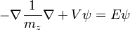
For the Schrodinger solver, it will use m_z to calculate the quantum confinement effects. The equation will solve |
For the Schrodinger solver, it will use m_z to calculate the quantum confinement effects. The equation will solve |
||
<math> {- \nabla \frac{1}{m_{z}} \nabla + V } \psi = E \psi </math> |
<math> {- \nabla \frac{1}{m_{z}} \nabla + V } \psi = E \psi </math> |
||
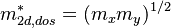
| − | + | For the n2d calculation, the density of state effective mass in the 2D structures is |
|
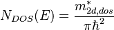
<math> m_{2d,dos}^{*} = ( m_{x} m_{y} ) ^{1/2} </math> |
<math> m_{2d,dos}^{*} = ( m_{x} m_{y} ) ^{1/2} </math> |
||
<math> N_{DOS}(E) = \frac{m_{2d,dos}^{*}}{\pi\hbar^{2}}</math> |
<math> N_{DOS}(E) = \frac{m_{2d,dos}^{*}}{\pi\hbar^{2}}</math> |
||
| − | For structures like Si, it may have some problems when Schrodinger solver is used. Since Si has six valleys with effective |
+ | For structures like Si, it may have some problems when the Schrodinger solver is used. Since Si has six valleys with effective masses in different directions (<math>m_{l}=0.98 m_{0}, m_{l}=0.19 m_{0}</math>, if we do not solve the Schrodinger equations, we can simply use m_e =1.08 m0 in the $1Dparameter. Or here, we can set |
$1Daddefmas |
$1Daddefmas |
||
1 |
1 |
||
| − | 0.49 0.49 0.49 0.16 0.16 0.16 0.98 0.19 0.19 6 |
+ | 0.49 0.49 0.49 1 0.0 0.16 0.16 0.16 1 0.0 '''0.98 0.19 0.19 6 0.0''' |
| − | For the Schrodinger solver, after |
+ | For the Schrodinger solver, after quantum confined effects, we can expect two confinement in the electron effective mass, the lower valleys are z valleys with mz=0.98, N=2. We can neglect the high valleys, and only two valleys are left as ground states. The setting would be |
$1Daddefmas |
$1Daddefmas |
||
1 |
1 |
||
| − | 0.49 0.49 0.49 0.16 0.16 0.16 0.98 0.19 0.19 2 |
+ | 0.49 0.49 0.49 0.16 0.0 0.16 0.16 0.98 0.0 0.19 0.19 2 0.0 |
<math> m_{2d,dos}^{*} = ( m_{x} m_{y} ) ^{1/2} (N)^{1/2}= 0.19 * \sqrt{2} * m_{0} </math> |
<math> m_{2d,dos}^{*} = ( m_{x} m_{y} ) ^{1/2} (N)^{1/2}= 0.19 * \sqrt{2} * m_{0} </math> |
||
<math> N_{DOS}(E) = \frac{m_{2d,dos}^{*}}{\pi\hbar^{2}}</math> |
<math> N_{DOS}(E) = \frac{m_{2d,dos}^{*}}{\pi\hbar^{2}}</math> |
||
| − | If we want to use type 2 to consider the second confine states, we can set |
+ | If we want to use type 2 to consider the second confine states, we can set ( Note x and y is undistinguished in 1D simulation program as they will be treated together) |
$1Daddefmas |
$1Daddefmas |
||
2 |
2 |
||
| − | 0.49 0.49 0.49 0.16 0.16 0.16 0.98 0.19 0.19 2 0.19 0.98 0.19 4 |
+ | 0.49 0.49 0.49 1 0.0 0.16 0.16 0.16 1 0.0 '''0.98 0.19 0.19 2 0.0 0.19 0.98 0.19 4 0.0''' |
| − | For unconfined conditions, it will set the mass of electron to be |
+ | For unconfined conditions, it will set the mass of the electron to be |
<math> m_{dos}^{*} = \left( (m_x m_y m_z)^{1/3})^{3/2} \times 2 + (m_x m_y m_z)^{1/3})^{3/2} \times 4 \right)^{2/3} </math> |
<math> m_{dos}^{*} = \left( (m_x m_y m_z)^{1/3})^{3/2} \times 2 + (m_x m_y m_z)^{1/3})^{3/2} \times 4 \right)^{2/3} </math> |
||
| 行 72: | 行 72: | ||
<math> m_{2d,dos,1}^{*} = ( m_{x} m_{y} ) ^{1/2} (N)^{1/2}= 0.19 * \sqrt{2} * m_{0} </math> |
<math> m_{2d,dos,1}^{*} = ( m_{x} m_{y} ) ^{1/2} (N)^{1/2}= 0.19 * \sqrt{2} * m_{0} </math> |
||
<math> m_{2d,dos,2}^{*} = ( m_{x} m_{y} ) ^{1/2} (N)^{1/2}= (0.19 * 0.98)^{1/2} \sqrt{4} * m_{0} </math> |
<math> m_{2d,dos,2}^{*} = ( m_{x} m_{y} ) ^{1/2} (N)^{1/2}= (0.19 * 0.98)^{1/2} \sqrt{4} * m_{0} </math> |
||
| + | |||
| + | For the In0.5Ga0.5P material, which has a 2nd valley (X) close to Gamma valley. In addition, the QB is usually dominated by X valley, which is an indirect bandgap. To solve Schrodinger equations, it is better to solve <math>\Gamma </math> valley and X separately. For Example, In0.5Ga0.5P is the direct bandgap X valley is above the <math>\Gamma </math> valley around 0.2eV, AlInP is the indirect bandgap, where X valley is below <math>\Gamma </math> valley about 0.4eV. Then we can use type 2 and set the first Ec as <math>\Gamma </math> valley and the 2nd Ec as X valley. Then |
||
| + | |||
| + | |||
| + | $1Daddefmas |
||
| + | 2 |
||
| + | 0.49 0.49 0.49 1 0.0 0.16 0.16 0.16 1 0.0 '''0.08 0.08 0.08 1 0.0 0.98 0.19 0.19 3 0.2''' -> InGaP |
||
| + | 0.49 0.49 0.49 1 0.0 0.16 0.16 0.16 1 0.0 '''0.098 0.098 0.098 1 0.4 0.94 0.21 0.21 3 0.0''' -> AlInP |
||
於 2023年3月11日 (六) 15:59 的最新修訂
$1Daddefmas is the function to add additional effective mass information for electron and holes. In some cases, the electron's (holes) effective mass in different directions are different. Hence the new functions is to put additional information for the program to calculate.
$1Daddefmas
I_effective_type


... to N layers

I_effective_type is the input type. The default should be 1. The typical semiconductor material has a heavy hole, a light hole, and electron effective mass of a direct band. The type 1 is used.
For I_effective_type= 1, m_{hh,z} ~~ m_{hh,x}~~ m_{hh,y}~~N_{valley}~~\Delta E_{hh}~~m_{lh,z} ~~ m_{lh,x}~~ m_{lh,y}~~N_{valley}~~\Delta E_{lh}~~m_{e,z} ~~ m_{e,x}~~ m_{hh,y}~~N_{valley}~~\Delta E_{c1}....</math>
For I_effective_type= 2,

Note: For type 2, it is designed for direct and indirect calculation in landscape cases.
z is the calculation direction of 1D program. If there is a QW, z is the confined direction in the 1D program.is the valley number of electrons
For example, for a material like GaN effective mass for HH is 1.8, LH=0.17, and the electron is 0.21 in the growth direction and 0.2 in the x,y direction. We set
 $1Daddefmas
 1
 1.8 1.8 1.8 1 0.0 0.17 0.17 0.17 1 0.0 0.21 0.2 0.2 1 0.0
 1.8 1.8 1.8 1 0.0 0.17 0.17 0.17 1 0.0 0.21 0.2 0.2 1 0.0
 1.8 1.8 1.8 1 0.0 0.17 0.17 0.17 1 0.0 0.21 0.2 0.2 1 0.0
 .... to N layers
Example II: For a material like AlGaN effective mass for HH is 1.8, LH=0.17, and the electron is 0.21 in the growth direction and 0.2 in the x,y direction. If it is under strain and HH shifts to the top first band by  (move up use positive sign),
 $1Daddefmas
 1
 1.8 1.8 1.8 1 0.2 0.17 0.17 0.17 1 0.0 0.21 0.2 0.2 1 0.0
 1.8 1.8 1.8 1 0.2 0.17 0.17 0.17 1 0.0 0.21 0.2 0.2 1 0.0
 1.8 1.8 1.8 1 0.2 0.17 0.17 0.17 1 0.0 0.21 0.2 0.2 1 0.0
 .... to N layers
For example, for a material effective mass for HH_growth direction is 1.4 in the other two directions are 0.7 and 0.9, LH=0.17, and electron is 0.3 in the growth direction and 0.1 in the x,y direction with 3 valleys, we set
 $1Daddefmas
 1
 1.4 0.7 0.9 1 0.0 0.17 0.17 0.17 1 0.0 0.3 0.1 0.1 3 0.0
 1.4 0.7 0.9 1 0.0 0.17 0.17 0.17 1 0.0 0.3 0.1 0.1 3 0.0
 1.4 0.7 0.9 1 0.0 0.17 0.17 0.17 1 0.0 0.3 0.1 0.1 3 0.0
 .... to N layers
Actually, the simulation program mainly uses the density of state effective mass. The different direction's effective mass will be put together as
For conduction band:
For the valence band
For the Schrodinger solver, it will use m_z to calculate the quantum confinement effects. The equation will solve
For the n2d calculation, the density of state effective mass in the 2D structures is
For structures like Si, it may have some problems when the Schrodinger solver is used. Since Si has six valleys with effective masses in different directions ( , if we do not solve the Schrodinger equations, we can simply use m_e =1.08 m0 in the $1Dparameter. Or here, we can set
 $1Daddefmas
 1
 0.49 0.49 0.49 1 0.0 0.16 0.16 0.16 1 0.0 0.98 0.19 0.19 6 0.0
For the Schrodinger solver, after quantum confined effects, we can expect two confinement in the electron effective mass, the lower valleys are z valleys with mz=0.98, N=2. We can neglect the high valleys, and only two valleys are left as ground states. The setting would be
 $1Daddefmas
 1
 0.49 0.49 0.49 0.16 0.0 0.16 0.16 0.98 0.0 0.19 0.19 2 0.0

If we want to use type 2 to consider the second confine states, we can set ( Note x and y is undistinguished in 1D simulation program as they will be treated together)
 $1Daddefmas
 2
 0.49 0.49 0.49 1 0.0 0.16 0.16 0.16 1 0.0 0.98 0.19 0.19 2 0.0 0.19 0.98 0.19 4 0.0
For unconfined conditions, it will set the mass of the electron to be

For the confined conditions, it will


For the In0.5Ga0.5P material, which has a 2nd valley (X) close to Gamma valley. In addition, the QB is usually dominated by X valley, which is an indirect bandgap. To solve Schrodinger equations, it is better to solve  valley and X separately. For Example, In0.5Ga0.5P is the direct bandgap X valley is above the valley around 0.2eV, AlInP is the indirect bandgap, where X valley is below valley about 0.4eV. Then we can use type 2 and set the first Ec as valley and the 2nd Ec as X valley. Then
 $1Daddefmas
 2
 0.49 0.49 0.49 1 0.0 0.16 0.16 0.16 1 0.0 0.08 0.08 0.08 1 0.0 0.98 0.19 0.19 3 0.2    -> InGaP
 0.49 0.49 0.49 1 0.0 0.16 0.16 0.16 1 0.0 0.098 0.098 0.098 1 0.4 0.94 0.21 0.21 3 0.0    -> AlInP